Bayesian Gaussian Processes with Uncertain Coordinates: A Mining Case Study

What the paper claims

• In many geoscience surveys the recorded drill‑hole coordinates are only approximate, often corrupted by meters of error.
• By treating the true coordinates (s_i) as latent variables and placing a Normal prior around the observed positions (\tilde{s}_i), the covariance function of a Gaussian process (GP) can be evaluated at the latent locations.
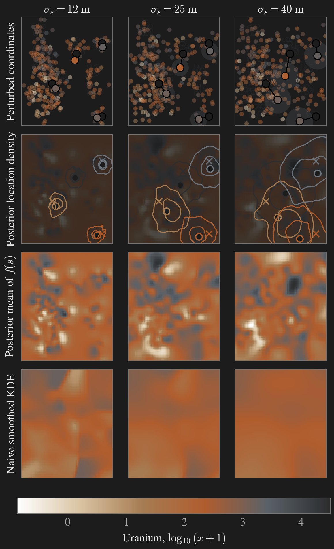
• Using PyMC’s gp.Marginal and a data container (pm.Data) the model can be refit quickly for several assumed error scales ((\sigma_s)).
• Experiments on the classic Walker Lake uranium‑vanadium dataset show that posterior predictions retain major spatial trends even when the coordinate error is large, while a naïve Nadaraya‑Watson kernel smoother fails to capture the same structure.

What is actually new

1. Latent‑location GP formulation – The idea of noisy inputs for GPs is not new; Cressie & Kornak (1990) and Cervone & Pillai (2002) discussed it in a geostatistical context. What this notebook adds is a clean PyMC implementation that swaps the observed coordinates on the fly via pm.set_data. The Δs ~ Normal(0, σ_s I) prior is fixed per experiment, turning the coordinate error into a hyper‑parameter that can be varied without redefining the model.
2. Marginalisation of the GP – By using pm.gp.Marginal, the latent GP values at the observations are analytically integrated out. This reduces the dimensionality of the sampling problem to the hyper‑parameters ((μ, σ, ℓ, σ_0)) and the coordinate offsets (Δs). The trade‑off is that the covariance matrix must be recomputed for every proposed (Δs), which makes each NUTS step expensive.
3. Empirical comparison – The notebook compares three error levels ((σ_s = 12, 25, 40) m). Posterior summaries show a steady increase in the mean displacement of the inferred true locations and a modest rise in the length‑scale (ℓ). Divergences and inflated (\hat{R}) values appear as the error grows, highlighting the practical limits of current HMC samplers for this model.
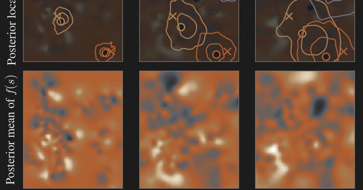
4. Visualization pipeline – The author builds a four‑panel figure for each error level: (i) perturbed observations, (ii) posterior high‑density contours for a handful of points, (iii) posterior mean of the latent field, and (iv) a naïve KDE surface. The figure (saved as error-in-location-grid.png) illustrates how uncertainty propagates from coordinates to the predicted surface.

Why it matters

• Mining and environmental monitoring often rely on sparse, expensive samples. Ignoring coordinate error can bias kriging estimates, especially when the error scale is comparable to the spatial correlation length.
• Bayesian treatment provides a principled way to propagate this uncertainty through to predictions, rather than applying a post‑hoc correction.
• The approach is model‑agnostic: any GP kernel (Matern, RBF, etc.) can be swapped, and the same data‑container trick works for other latent covariates (e.g., uncertain depth or time).

Limitations and practical concerns

1. Computational cost – Each HMC iteration requires rebuilding the full covariance matrix for the current (X_{true}). With 200‑plus observations the runtime climbs to several hours per chain, as reported (≈ 2 h per run). Scaling to thousands of points would need sparse GP approximations or inducing‑point methods, which are not explored here.
2. Sampler diagnostics – The notebook reports many divergent transitions and (\hat{R}) values above 1.01 for larger (σ_s). This suggests the posterior geometry becomes highly curved; re‑parameterising the offset (e.g., non‑centered) or using a more aggressive target_accept could improve stability.
3. Fixed error variance – Treating (σ_s) as known sidesteps the question of how to learn the true measurement error from the data. A hierarchical prior on (σ_s) would be more realistic but would add another difficult dimension to the sampler.
4. Comparison baseline – The naïve kernel smoother is a harsh baseline. More competitive alternatives (e.g., kriging with measurement‑error models, or GP regression with input‑noise approximations such as the variational approach of McHutchon & Rasmussen, 2011) are not included, limiting the strength of the claim that the Bayesian GP “outperforms” simpler methods.

Take‑away for practitioners

• If you have few hundred samples and can afford a few hours of HMC, modelling coordinate error explicitly can reveal how much spatial structure survives noisy positioning.
• For larger datasets, consider sparse GP frameworks (e.g., GPyTorch’s VariationalStrategy) and non‑centered parametrisations for the latent coordinates to keep sampling efficient.
• Always check diagnostics: divergences and low effective sample sizes are early warnings that the posterior is not being explored adequately.

Further reading

• Cressie, N., & Kornak, J. (1990). Spatial statistics with measurement error. Journal of the Royal Statistical Society.
• Cervone, D., & Pillai, N. S. (2002). Kriging with uncertain locations. Environmetrics.
• McHutchon, A., & Rasmussen, C. (2011). Gaussian Process Training with Input Noise. NIPS.

Code and data

• The Walker Lake dataset is bundled with the R package gstat and can be accessed via the gstat GitHub mirror: https://github.com/cran/gstat
• Full notebook implementation (including the figure) is available at the author’s GitHub: https://github.com/ckrapu/uncertain-location-gp

Bottom line The notebook demonstrates a clean Bayesian workflow for handling uncertain spatial inputs, but the method’s scalability and sampler robustness remain open challenges. For real‑world mining projects, the approach is worth a trial on modest‑size datasets, while larger surveys will need approximations or more sophisticated inference strategies.