Smoothed polygons

The squircle, a shape intermediate between a square and a circle, is defined by the Lp norm equation |x|^p + |y|^p = 1, where p=2 yields a Euclidean circle, p approaching infinity yields a square, and p=4 is the conventional parameter for a squircle. This shape has found widespread use in design, computer graphics, and user interface elements due to its smooth, rounded appearance that avoids the harsh corners of a square while retaining its general rectangular form.

The previous post in this series, available on John D Cook's blog, extended this concept to triangular symmetry, creating a shape that interpolates between an equilateral triangle and a Euclidean circle. This triangular squircle was constructed using three functions L_i(x,y), each corresponding to one side of a reference triangle, where the level set L_i(x,y) = 1 defines each triangular side. A soft penalty function, measuring deviation of each L_i from 1, was summed across all three sides, with level sets of this combined penalty producing the rounded triangular shapes.

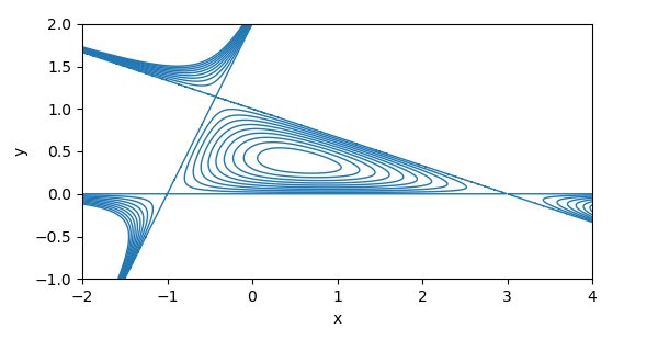
An alternative construction, outlined here, adjusts the definition of the L_i functions so that each triangular side is defined by the level set L_i(x,y) = 0 rather than L_i = 1. This shift leverages a fundamental algebraic property, that the product of three numbers equals zero if and only if at least one of the numbers is zero. Defining a combined function f(x,y) = L_1(x,y) * L_2(x,y) * L_3(x,y), the zero level set f(x,y) = 0 corresponds exactly to the union of the three triangular sides, i.e., the boundary of the reference triangle. For small positive values of c, the level sets f(x,y) = c are smooth curves that approximate the triangle, as long as the gradient of f is non-zero at all points on the level set. Since f = c ≠ 0 implies none of the L_i are zero, the gradient calculation avoids the corner points where two L_i vanish simultaneously, which are the vertices of the original triangle.

The gradient of f is given by the sum L_2L_3∇L_1 + L_1L_3∇L_2 + L_1L_2∇L_3. For c ≠ 0, all L_i are non-zero, so each term in the sum is well-defined, but this does not guarantee a non-zero gradient everywhere. For regular polygons, the normals ∇L_i sum to zero when weighted equally, leading to gradient zeros at the centroid of the triangle where all L_i take equal value. This results in a critical point at the center of the level set, which can cause local flattening or non-smoothness in the approximated shape, a trade-off not present in the penalty-based approach.

This method is not limited to triangles. Any polygon, convex or concave, can be approximated by defining a linear function L_i for each side, then taking the product of all L_i as the combined function f. Level sets of f = c for small c will produce smooth approximations of the polygon, with the same trade-offs in connectivity and gradient consistency. The approach also extends to shapes bounded by curved arcs, where each L_i is replaced by a function defining a curved boundary segment, and the product of these functions yields smooth approximations of the curved shape.

A key caveat of the product approach is that level sets for c > 0 are not necessarily connected. Since the product f is positive in regions where an even number of L_i are negative (for polygons where L_i is positive inside the shape), the level set f = c will include components inside the original polygon, where all L_i are positive, as well as components outside the polygon where two L_i are negative (for triangular cases). Practitioners must select the connected component corresponding to the interior of the original polygon to obtain the desired smoothed shape, adding a post-processing step not required for penalty-based methods where level sets are typically connected.

The product-based method offers several advantages for practical applications. In computer graphics, smooth polygon approximations are used for anti-aliasing, procedural shape generation, and physics simulations where sharp corners can cause numerical instability. The algebraic construction is easily parameterized, allowing for adjustable smoothing by changing the value of c, and generalizes seamlessly to arbitrary polygons without custom penalty function design. For CAD software, this method provides a way to smooth imported polygonal meshes while retaining the underlying topological structure of the original shape. In machine learning, smooth shape priors for image segmentation can leverage this construction to create differentiable shape approximations that are easier to optimize than sharp-edged polygons.

Comparing the two methods, the penalty-based approach from the previous post avoids the connectivity issues of the product method, as the sum of penalty functions typically produces a single connected level set for all c. However, the penalty approach requires tuning the penalty function for each L_i, and the resulting shape may not align as closely with the original polygon's topology, as the penalty sum does not directly encode the union of sides. The product method's alignment with the algebraic structure of polygon boundaries makes it more intuitive for theoretical work in computational geometry, even with the added complexity of component selection.

The development of smoothed polygon approximations via product functions highlights the interplay between algebraic topology and computational shape design. While the method introduces practical considerations around connectivity and gradient consistency, its generalizability and intuitive construction make it a valuable addition to the toolkit for working with smooth shape approximations, building on the foundational work of squircles and their polygonal analogs.