When incident.io's alert filtering API hit a P95 latency of 5s, a team turned to a niche computer science trick—the Bloom filter—to achieve a 16x performance boost, transforming a sluggish user experience into a seamless one.
At AWS re:Invent, the team at incident.io unveiled a deep dive into a critical performance optimization that transformed their platform. By leveraging a probabilistic data structure known as a Bloom filter, they improved the P95 latency of a key API endpoint from a sluggish 5 seconds to a blistering 0.3 seconds. This wasn't just a speed bump; it was a fundamental rethink of how they handle large-scale data filtering, with profound implications for developers and platform architects dealing with similar challenges.
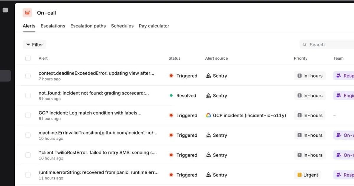
The core of their On-call product is Alerts, messages received from customers' monitoring systems like Alertmanager or Datadog. These alerts are stored in a comprehensive database table, providing customers with a full history for debugging and trend analysis. To make this data navigable, incident.io built a powerful filtering UI, allowing users to narrow down millions of alerts by source, priority, team, and custom features.
However, as incident.io onboarded larger organizations generating millions of alerts, this powerful feature became a performance bottleneck. Users reported waits of up to 12 seconds, with the P95 response time for large organizations hovering at 5 seconds. Every page load, filter update, or scroll triggered an agonizing wait for a loading spinner, undermining the platform's value.
The Bottleneck: A Naive Approach to Filtering
The root of the problem lay in their initial algorithm for fetching filtered results. Alerts are stored in a Postgres table with a simplified structure:
| id | organisation_id | priority | ... | attribute_values (JSONB) |
|---|
First-class dimensions like priority have their own columns, but custom attributes—such as team and feature—are stored as key-value pairs in a JSONB column. The filtering process worked like this:
- Initial DB Fetch: The application would fetch a large batch of rows (e.g., 500) from the database using an index on
(organisation_id ASC, id DESC). - In-Memory Deserialization: The Object-Relational Mapper (ORM) would deserialize these rows into Go structs. Crucially, it would also deserialize the
JSONBattribute_valuesfor each row into more complex structs. - In-Memory Filtering: The application would then iterate through the 500 deserialized objects and apply the custom attribute filters in memory.
- Repeat: If the batch didn't contain enough matching alerts (e.g., the target was 50), the process would repeat with another SQL query until the page was full.
This approach was highly inefficient. Telemetry revealed that fetching and deserializing a batch of 500 rows took approximately 500ms, with only 50ms of that time spent waiting for the database query itself. The majority of the time was spent on CPU-intensive deserialization of JSONB data in the application layer. Furthermore, as the number of alerts grew, the worst-case scenario—where few rows were filtered out by the database—required fetching and processing many such batches, causing latency to spiral.
The Search for a Solution: Pushing Filtering to the Database
The bottleneck was clear: fetching and deserializing large amounts of data from Postgres. The solution, therefore, was to push as much of the filtering logic as possible into the database itself. The team explored two primary options.
Option 1: The Standard Solution – A GIN Index
The conventional Postgres approach for indexing complex types like JSONB is a GIN (Generalized Inverted Index). They could create a GIN index on the attribute_values column using the jsonb_path_ops operator class. This would allow Postgres to efficiently perform full-text searches and path queries on the JSON data.
Option 2: The Niche Trick – Bloom Filters
This was a proposal from Lawrence Jones, one of incident.io's founding engineers. A Bloom filter is a space-efficient, probabilistic data structure that tests whether an element is a member of a set. It can answer one of two questions:
- "No": The element is definitely not in the set.
- "Maybe": The element is possibly in the set.
In exchange for this probabilistic nature, Bloom filters offer extremely fast query times and low memory overhead. An item is added to a Bloom filter by hashing it with several different functions to produce bit positions in a bitmap, which are then set to 1. To check for an item's presence, the same hash functions are used. If all the corresponding bits in the bitmap are 1, the item might be in the set. If any bit is 0, the item is definitely not.
The team saw an opportunity. They could represent an alert's custom attributes as a set of strings (e.g., {"team":"oncall", "feature":"alerts"}). A search for alerts with a specific attribute value, then, becomes a set membership test. By encoding this set into a Bloom filter and storing the resulting bitmap in the database, they could let Postgres perform a rapid, bitwise "one of" operation to filter rows before they were ever sent to the application.
The Implementation: Encoding Attributes and Measuring Performance
The team implemented the Bloom filter solution by:
- Encoding Attribute Values: Representing each key-value pair in the
attribute_valuesJSONB as a string (e.g.,"team:oncall"and"feature:alerts"). - Generating Bitmaps: For each alert, they computed a 512-bit bitmap using seven different hashing functions. This configuration was mathematically tuned to achieve a target false positive rate of just 1%.
- Storing the Bitmap: They added a new column,
attribute_values_bitmap, of typebit(512)to their alerts table and populated it with the computed bitmaps. - Querying with Bitwise Logic: When filtering, they generated a
bitmaskfor the desired attributes. The SQL query then used a bitwise AND operation (&) to find rows where the stored bitmap contained the bitmask.
With this in place, their new query for "alerts with a priority of urgent or critical, assigned to the On-call team, affecting the alerts feature" looked like this:
SELECT * FROM alerts
WHERE organisation_id = ?
  AND priority IN ('urgent', 'critical')
  AND attribute_values_bitmap & bitmask = bitmask
ORDER BY id DESC
LIMIT 50;
The 1% false positive rate meant they still had to perform a final in-memory check on the returned results to eliminate false matches, but this was a tiny fraction of the previous deserialization workload.
The Spike: GIN vs. Bloom Filter
The team prototyped both options and tested them against two scenarios on a table with ~1 million alerts:
- Frequent Alerts: A query matching ~500,000 alerts.
- Infrequent Alerts: A query matching only ~500 alerts.
The results were telling:
- GIN Index: For infrequent matches, the GIN index was incredibly fast. However, for frequent matches, its performance degraded significantly. The query planner had to read and sort all 500,000 matching rows before applying the
LIMIT 50clause, wasting immense I/O and CPU. - Bloom Filter: The bloom filter's performance was the inverse. It was slower for infrequent matches because it had to scan a larger portion of the index to find enough candidates. But for frequent matches, it was exceptionally fast, as it could quickly discard non-matching rows.
Both options scaled with the total number of alerts, a critical flaw for a system designed to retain a complete history. This led to a final, crucial insight.
The Final Piece: Leveraging Recency Bias
The team realized they were fighting against a natural user behavior: customers are typically interested in their most recent alerts. Yet, their queries were scanning the entire history of an organization's alerts, from the very first one to the present.
The solution was simple yet powerful: they made the created_at filter mandatory and set a default value of 30 days. This was a product decision rooted in technical reality. By partitioning the search space to the last 30 days, they drastically reduced the number of rows any query had to examine.
With this change, both the GIN and Bloom filter queries became dramatically more efficient. The GIN index could now use a composite index, and the Bloom filter could leverage the existing pagination index on (organisation_id, id DESC) since ULIDs (their unique ID format) are lexicographically sortable by time.
The Decision and the Outcome
With performance now excellent for both frequent and infrequent queries within the 30-day window, the team faced a final choice: which solution to implement? The debate was "robust" but centered on maintainability and risk.
- GIN Index Concerns: GIN indexes can be large, both on disk and in memory, and have high write overhead. There was a risk that as the index grew, it could consume too much of Postgres's shared buffers, negatively impacting other parts of the platform.
- Bloom Filter Concerns: Bloom filters are a niche topic. The team worried that the custom implementation would be difficult for future engineers to understand and maintain. They were also hesitant to essentially build their own indexing mechanism when a database is supposed to handle that.
Ultimately, they chose the Bloom filter. Their decision was driven by a desire to avoid future rework. They were more confident that the Bloom filter, despite its complexity, was a solution they would only need to build once.
The combined impact of the Bloom filter and the mandatory 30-day time bound was staggering. The P95 response time for large organizations improved from 5 seconds to 0.3 seconds—a 16x performance boost. Their powerful, slick filtering was slick again, and with a scalable architecture, it would remain so as they continued to onboard customers who now generate over a million alerts per week.
This case study is a prime example of how deep technical thinking and product understanding must go hand in hand. The Bloom filter provided the raw computational power, but the insight into user behavior—leveraging recency bias—provided the context to make that power truly effective. For developers and architects facing similar challenges with large-scale data filtering, it's a powerful reminder that the best solutions often lie at the intersection of clever algorithms and a pragmatic understanding of how your software is actually used.
"This is a great example of how technical and product thinking can go hand in hand. However you go about it, this is one of those hard technical problems to solve, and I’m lucky to work alongside incredibly talented engineers. However, understanding our customers and how they use our product led us to a vital piece of the puzzle. We needed both to really nail this."
— Source: incident.io Engineering Blog
Comments
Please log in or register to join the discussion