Understanding Lagrange Interpolating Polynomials: A Deep Dive

Polynomial interpolation is a fundamental technique in numerical analysis that finds a polynomial function fitting a given set of data points perfectly. When we have distinct points and want to find polynomial coefficients such that the polynomial passes through all these points, Lagrange interpolation offers an elegant solution.

The Linear Algebra Approach

When we assign all points into a generic polynomial, we get a system of linear equations that can be represented by a matrix equation. The matrix on the left is called the Vandermonde matrix, which is known to be invertible when the points are distinct. This guarantees a single solution that can be calculated by inverting the matrix.

However, the Vandermonde matrix is often numerically ill-conditioned, making direct inversion impractical for real-world applications. Several better methods exist for computing the interpolating polynomial.

The Lagrange Basis Functions

The Lagrange interpolation polynomials emerge from a simple yet powerful idea. Let's define the Lagrange basis functions as follows, given our points:

$$l_i(x) = \prod_{j=0, j\neq i}^{n} \frac{x - x_j}{x_i - x_j}$$

In words, $l_i$ is constrained to 1 at $x_i$ and to 0 at all other $x_j$ where $j \neq i$. We don't care about its value at any other point.

The linear combination:

$$p(x) = \sum_{i=0}^{n} y_i l_i(x)$$

is then a valid interpolating polynomial for our set of points, because it's equal to $y_i$ at each $x_i$.

A Concrete Example

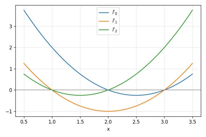
Let's use a concrete example to visualize this. Suppose we have the following set of points we want to interpolate: $(1,4), (2,2), (3,3)$. We can calculate $l_0(x)$, $l_1(x)$, and $l_2(x)$, and get the following functions:

Note where each intersects the axis. These functions have the right values at all $x_j \neq i$. If we normalize them to obtain $l_i(x)$, we get these functions:

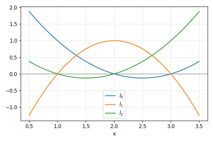
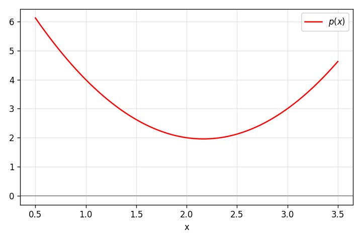
Note that each polynomial is 1 at the appropriate $x_i$ and 0 at all the other $x_j$, as required. With these $l_i(x)$, we can now plot the interpolating polynomial $p(x) = \sum_{i=0}^{2} y_i l_i(x)$, which fits our set of input points:

Polynomial Degree and Uniqueness

We've just seen that the linear combination of Lagrange basis functions:

$$p(x) = \sum_{i=0}^{n} y_i l_i(x)$$

is a valid interpolating polynomial for a set of distinct points. What is its degree? Since the degree of each $l_i$ is $n$, then the degree of $p$ is at most $n$.

We've just derived the first part of the Polynomial interpolation theorem: for any data points where no two are the same, there exists a unique polynomial of degree at most $n$ that interpolates these points.

Proving Uniqueness

We've demonstrated existence and degree, but not yet uniqueness. So let's turn to that. We know that $p$ interpolates all points, and its degree is at most $n$. Suppose there's another such polynomial $q$. Let's construct:

$$r(x) = p(x) - q(x)$$

What do we know about $r$? First of all, its value is 0 at all our $x_i$, so it has $n+1$ roots. Second, we also know that its degree is at most $n$ (because it's the difference of two polynomials of such degree).

These two facts are a contradiction. No non-zero polynomial of degree at most $n$ can have $n+1$ roots (a basic algebraic fact related to the Fundamental theorem of algebra). So $r$ must be the zero polynomial; in other words, our $p$ is unique.

Lagrange Polynomials as a Basis

The set $\mathcal{P}_n$ consists of all real polynomials of degree at most $n$. This set - along with addition of polynomials and scalar multiplication - forms a vector space. We called the "Lagrange basis" previously, and they do - in fact - form an actual linear algebra basis for this vector space.

To prove this claim, we need to show that Lagrange polynomials are linearly independent and that they span the space.

Linear Independence

We have to show that $\sum_{i=0}^{n} c_i l_i(x) = 0$ implies all $c_i = 0$. Recall that $l_i$ is 1 at $x_i$, while all other $l_j$ where $j \neq i$ are 0 at that point. Therefore, evaluating at $x_i$, we get:

$$\sum_{j=0}^{n} c_j l_j(x_i) = c_i \cdot 1 + \sum_{j\neq i} c_j \cdot 0 = c_i$$

Since this equals 0, we have $c_i = 0$. Similarly, we can show that $c_j = 0$ for all $j$.

Span

We've already demonstrated that the linear combination of $l_i(x)$:

$$p(x) = \sum_{i=0}^{n} y_i l_i(x)$$

is a valid interpolating polynomial for any set of distinct points. Using the polynomial interpolation theorem, this is the unique polynomial interpolating this set of points. In other words, for every $p \in \mathcal{P}_n$, we can identify any set of distinct points it passes through, and then use the technique described in this post to find the coefficients of $p$ in the Lagrange basis. Therefore, the set spans the vector space $\mathcal{P}_n$.

The Interpolation Matrix in Lagrange Basis

Previously we've seen how to use the monomial basis to write down a system of linear equations that helps us find the interpolating polynomial. This results in the Vandermonde matrix. Using the Lagrange basis, we can get a much nicer matrix representation of the interpolation equations.

Recall that our general polynomial using the Lagrange basis is:

$$p(x) = \sum_{i=0}^{n} c_i l_i(x)$$

Let's build a system of equations for each of the points. For $x_0$:

$$p(x_0) = \sum_{i=0}^{n} c_i l_i(x_0)$$

By definition of the Lagrange basis functions, all $l_i$ where $i \neq 0$ are 0, while $l_0$ is 1. So this simplifies to:

$$p(x_0) = c_0$$

But the value at node $x_0$ is $y_0$, so we've just found that $c_0 = y_0$. We can produce similar equations for the other nodes as well, $c_1 = y_1$, etc. In matrix form:

$$\begin{bmatrix} 1 & 0 & 0 & \cdots & 0 \ 0 & 1 & 0 & \cdots & 0 \ 0 & 0 & 1 & \cdots & 0 \ \vdots & \vdots & \vdots & \ddots & \vdots \ 0 & 0 & 0 & \cdots & 1 \end{bmatrix} \begin{bmatrix} c_0 \ c_1 \ c_2 \ \vdots \ c_n \end{bmatrix} = \begin{bmatrix} y_0 \ y_1 \ y_2 \ \vdots \ y_n \end{bmatrix}$$

We get the identity matrix; this is another way to trivially show that $c_i = y_i$, and so on.

Appendix: The Vandermonde Matrix

Given some numbers $x_0, x_1, \ldots, x_n$, a matrix of this form:

$$V = \begin{bmatrix} 1 & x_0 & x_0^2 & \cdots & x_0^n \ 1 & x_1 & x_1^2 & \cdots & x_1^n \ 1 & x_2 & x_2^2 & \cdots & x_2^n \ \vdots & \vdots & \vdots & \ddots & \vdots \ 1 & x_n & x_n^2 & \cdots & x_n^n \end{bmatrix}$$

Is called the Vandermonde matrix. What's special about a Vandermonde matrix is that we know it's invertible when $x_i$ are distinct. This is because its determinant is known to be non-zero. Moreover, its determinant is:

$$\det(V) = \prod_{0 \leq i < j \leq n} (x_j - x_i)$$

Here's why. To get some intuition, let's consider some small-rank Vandermonde matrices. Starting with a 2-by-2:

$$V_2 = \begin{bmatrix} 1 & x_0 \ 1 & x_1 \end{bmatrix}$$

$$ \det(V_2) = x_1 - x_0 $$

Let's try 3-by-3 now:

$$V_3 = \begin{bmatrix} 1 & x_0 & x_0^2 \ 1 & x_1 & x_1^2 \ 1 & x_2 & x_2^2 \end{bmatrix}$$

We can use the standard way of calculating determinants to expand from the first row:

$$ \det(V_3) = x_1 x_2^2 - x_2 x_1^2 - x_0 x_2^2 + x_2 x_0^2 + x_0 x_1^2 - x_1 x_0^2 $$

Using some algebraic manipulation, it's easy to show this is equivalent to:

$$ \det(V_3) = (x_1 - x_0)(x_2 - x_0)(x_2 - x_1) $$

For the full proof, let's look at the generalized $n$-by-$n$ matrix again:

$$V_n = \begin{bmatrix} 1 & x_0 & x_0^2 & \cdots & x_0^n \ 1 & x_1 & x_1^2 & \cdots & x_1^n \ 1 & x_2 & x_2^2 & \cdots & x_2^n \ \vdots & \vdots & \vdots & \ddots & \vdots \ 1 & x_n & x_n^2 & \cdots & x_n^n \end{bmatrix}$$

Recall that subtracting a multiple of one column from another doesn't change a matrix's determinant. For each column $j$ where $j \geq 2$, we'll subtract the value of column $j-1$ multiplied by $x_0$ from it (this is done on all columns simultaneously). The idea is to make the first row all zeros after the very first element:

$$V_n' = \begin{bmatrix} 1 & 0 & 0 & \cdots & 0 \ 1 & x_1 - x_0 & x_1^2 - x_0 x_1 & \cdots & x_1^n - x_0 x_1^{n-1} \ 1 & x_2 - x_0 & x_2^2 - x_0 x_2 & \cdots & x_2^n - x_0 x_2^{n-1} \ \vdots & \vdots & \vdots & \ddots & \vdots \ 1 & x_n - x_0 & x_n^2 - x_0 x_n & \cdots & x_n^n - x_0 x_n^{n-1} \end{bmatrix}$$

Now we factor out $(x_1 - x_0)$ from the second row (after the first element), $(x_2 - x_0)$ from the third row and so on, to get:

$$V_n' = \begin{bmatrix} 1 & 0 & 0 & \cdots & 0 \ 1 & 1 & x_1 & \cdots & x_1^{n-1} \ 1 & 1 & x_2 & \cdots & x_2^{n-1} \ \vdots & \vdots & \vdots & \ddots & \vdots \ 1 & 1 & x_n & \cdots & x_n^{n-1} \end{bmatrix} \cdot \prod_{j=1}^{n} (x_j - x_0)$$

Imagine we erase the first row and first column of $V_n'$. We'll call the resulting matrix $V_{n-1}'$. Because the first row of $V_n'$ is all zeros except the first element, we have:

$$\det(V_n') = \det(V_{n-1}') \cdot \prod_{j=1}^{n} (x_j - x_0)$$

Note that the first row of $V_{n-1}'$ has a common factor of $(x_1 - x_0)$, so when calculating $\det(V_{n-1}')$, we can move this common factor out. Same for the common factor of the second row, and so on. Overall, we can write:

$$\det(V_n') = \det(V_{n-1}') \cdot \prod_{j=1}^{n} (x_j - x_0) = \det(V_{n-2}') \cdot \prod_{j=2}^{n} (x_j - x_1) \cdot \prod_{j=1}^{n} (x_j - x_0)$$

But the smaller matrix $V_{n-1}'$ is just the Vandermonde matrix for $x_1, x_2, \ldots, x_n$. If we continue this process by induction, we'll get:

$$\det(V_n) = \prod_{0 \leq i < j \leq n} (x_j - x_i)$$

If you're interested, the Wikipedia page for the Vandermonde matrix has a couple of additional proofs.