Notes on Pretraining Parallelisms and Failed Training Runs

Training large language models has become an increasingly complex endeavor, with numerous technical challenges that can lead to failed pretraining runs. This article examines common failure modes and strategies for parallelizing training across multiple GPUs based on discussions with industry experts and technical lectures.

Why Pretraining Runs Fail

Breaking Causality in Expert Routing

One significant issue in modern transformer architectures is the breaking of causality during expert routing in models with sparse MoE (Mixture of Experts) components. When implementing expert routing, two primary approaches exist:

1. Token routing: Each token is allocated to its top-k experts based on router scores
2. Expert choice: Tokens are distributed to ensure each expert receives roughly an equal number of tokens

While expert choice prevents the wildly unbalanced allocation that can plague token routing, it introduces a critical problem: breaking causality. In expert choice, which expert a token gets allocated to may depend on which subsequent tokens (token n+k) would be routed to that expert. This creates a dependency that doesn't exist during inference, where causality must be preserved.

This issue may explain why some highly anticipated models, like Llama 4, have underperformed expectations. The model may have been trained with expert choice during training but deployed with token routing during inference, creating a distribution mismatch.

Another causality-breaking issue is token dropping, where experts ignore tokens in the batch that don't rank strongly enough. This can cause earlier tokens to be dropped based on the presence of later, more strongly-matched tokens, again violating the causal structure present during inference. This reportedly affected Gemini 2 Pro.

Numerical Precision Issues

Beyond architectural problems, numerical precision errors can significantly impact training outcomes. A notable example from early GPT-4 training involved the use of FP16 on collectives like all-reduce operations.

FP16 precision distributes its granularity according to logarithmic density - between 1 and 2, the mantissa bits carve the interval approximately 0.001 apart. However, at values of 1024 and above, the mantissa might be carving intervals by multiple whole number values. This creates a situation where adding 1 to 1024 might round back down to 1024, causing the calculated value to be orders of magnitude off the true value when summing many small gradients into a large accumulator.

Such bugs are particularly insidious because they don't cause immediate failures but rather subtly corrupt the training process, leading to suboptimal results that may not be detected until much later in the training process.

Implications for AI Training Reliability

These failure modes raise important questions about the reliability of AI training at scale. One perspective suggests there might be a finite number of fundamental failure modes, implying that once these are addressed, training runs could become more predictable. However, experts interviewed suggest the opposite - that as models scale, new bespoke issues will continue to emerge.

This has implications for automation efforts in AI training, particularly around kernel optimization. While some believe that kernel writing could be fully automated through reinforcement learning, given its verifiable nature, the complexity of optimizing for new hardware architectures (like Nvidia's Blackwell) suggests this may be more challenging than anticipated.

Furthermore, there's an important distinction between inference for RL generation versus end-user generation. Numerical drift between inference and training engines can cause subtle off-policy biases that significantly impact high-quality training but aren't issues for serving users.

Pretraining Parallelisms

The Basic Challenge

The fundamental equation for pretraining compute is straightforward:

Pretraining FLOPs = 6ND

Where N is the number of parameters and D is the number of tokens. This breaks down as:

• 2 FLOPs per parameter per token for the forward pass (multiply + add)
• 4 FLOPs per parameter per token for the backward pass (computing gradients)

As models grow larger, single-GPU training becomes impossible, requiring parallelization strategies.

Data Parallelism

The most straightforward approach is data parallelism, where model weights are copied across each GPU, and each GPU processes a portion of the batch. However, this approach quickly hits memory limitations as models grow larger, as each GPU must store the entire model.

Fully Sharded Data Parallelism (FSDP)

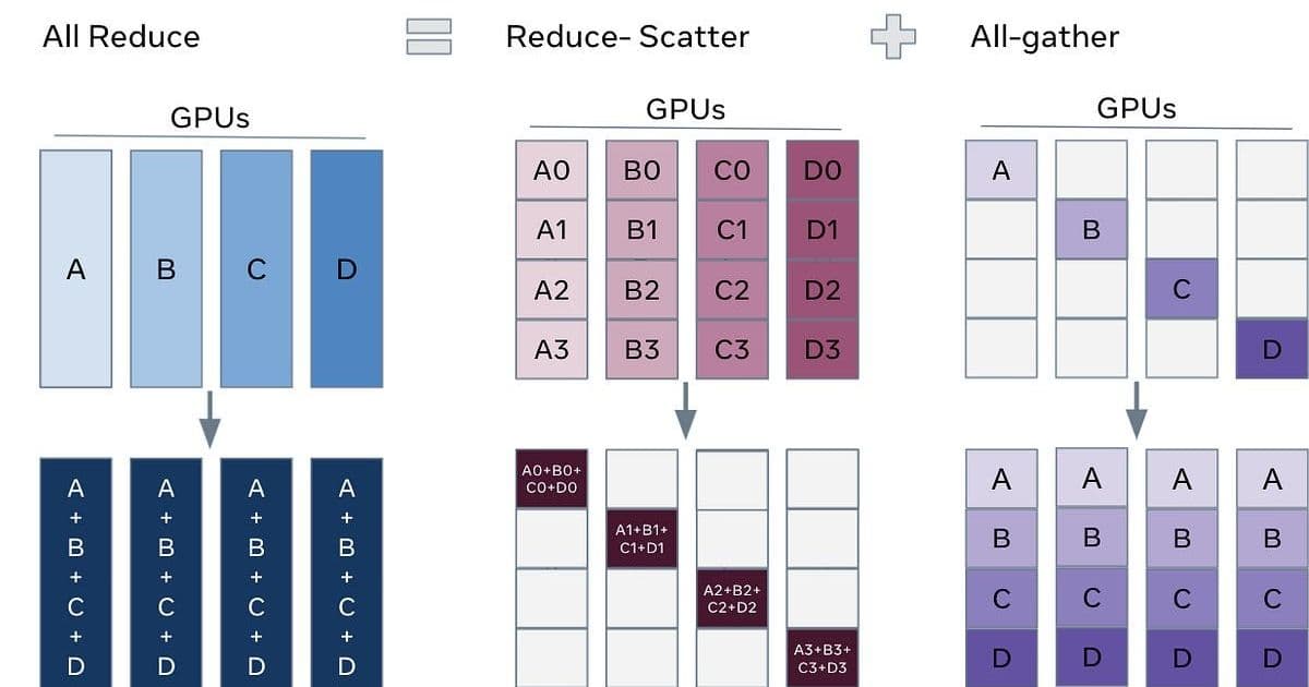
Fully Sharded Data Parallelism (FSDP) addresses memory limitations by distributing each layer's parameters across all GPUs. Each GPU stores only 1/N of each layer's parameters. Before processing each layer, an all-gather operation retrieves the full layer's parameters from all GPUs. After processing, the gathered parameters are discarded.

FSDP has become the default approach for several reasons:

1. Trivial compute-communication overlap: Since weights being communicated aren't dependent on the previous layer's computation, the next layer's weights can be gathered while the current layer is being processed.
2. Communication efficiency: While it may seem expensive to all-gather full layer weights, this is offset by the fact that regular data parallelism requires all-reduce operations for gradients after each backward pass. An all-gather has half the communication volume of an all-reduce.

The communication overhead for FSDP is approximately 3× the number of parameters (all-gather forward and backward, plus reduce-scatter for gradients), which is a 50% overhead over vanilla data parallelism.

Communication Crossover and Scaling Limits

Despite its advantages, FSDP isn't infinitely scalable. The fundamental issue is the communication crossover point, where communication time exceeds computation time, causing the model's MFU (Model Flops Utilization) to plummet.

• Compute time = (6 × # tokens × active params) / (compute per GPU × number of GPUs)
• Communication time = (# total params × 3) / (NVLink domain size × InfiniBand bandwidth)

As the number of GPUs increases, compute time decreases while communication time remains constant, eventually leading to the crossover point. At this point, additional parallelism strategies are needed.

Several factors affect the crossover point:

• Increasing batch size moves the crossover point to the right (more favorable)
• Making the model more sparse moves the crossover point to the left (less favorable)

TPUs are particularly well-suited for FSDP because they allow more accelerators within a domain, reducing communication overhead.

Batch Size Floor Limitation

FSDP faces a fundamental limitation related to batch size. Since attention is computed within sequences and can't be easily split across GPUs, there's a minimum batch size per GPU. For example, with a critical batch size of 10M tokens and sequence length of 10K, only 1K sequences are available, limiting scaling to 1K GPUs even with ample communication bandwidth.

Pipeline Parallelism

When FSDP reaches its scaling limits, pipeline parallelism is typically added. However, pipeline parallelism introduces its own challenges:

1. Pipeline bubbles: At the beginning of a batch, GPUs dedicated to final layers are underutilized, while at the end of the batch, GPUs dedicated to initial layers are underutilized.
2. Architecture constraints: Techniques like Kimi's attention-to-residuals (where each block attends to all previous layers' residuals) become difficult when residuals live on different pipeline stages.
3. Research iteration slowdown: The complexity of managing these parallelism strategies slows down research iteration, which is a significant cost in the fast-moving field of AI.

Optimizing Communication Hierarchically

To mitigate communication bottlenecks across multiple NVLink domains, hierarchical collective operations can be employed:

1. Reduce-scatter within a domain to give each GPU domain-level reduced gradients for a shard of the layer
2. All-reduce these shards across corresponding GPUs across domains
3. All-gather within a domain

This approach maximizes the use of available interconnect bandwidth by performing as much communication as possible within a domain before moving across domains.

Conclusion

The challenges in large-scale model training highlight the complexity of the problem beyond simply scaling compute. Issues like breaking causality in expert routing, numerical precision errors, and communication bottlenecks all represent significant hurdles that can lead to failed pretraining runs or suboptimal models.

As models continue to scale, it's likely that new technical challenges will emerge, requiring increasingly sophisticated parallelism strategies and careful attention to the subtle details that can make the difference between successful and failed training runs. This complexity suggests that fully automating kernel writing and other aspects of training optimization may be more challenging than some optimistic projections suggest.