Spatial Indexing at Scale: Why Uber Chose Hexagons Over Grids for Real-Time Driver Matching

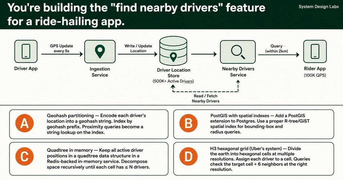
Building a "find nearby drivers" feature sounds straightforward until you scale it. At 500,000 active drivers updating GPS coordinates every 5 seconds, you're processing 100,000 proximity queries per second. The naive SQL approach that works at 1,000 drivers becomes a full table scan disaster at scale, pushing latency to 800ms while riders stare at spinners and drivers miss trip opportunities.

The core problem isn't just storing locations. It's maintaining real-time spatial indexes under extreme write pressure while serving sub-50ms read queries. Every solution involves trade-offs between write amplification, query accuracy, boundary handling, and operational complexity.

The Four Contenders

A) Geohash Partitioning

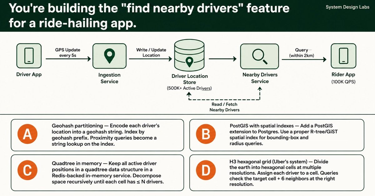
Geohash encodes latitude/longitude into a string where prefix matching approximates proximity. You index by geohash prefix, and proximity queries become string lookups.

The appeal: Simple to implement, works with any database, no extensions required.

The trap: Geohash uses a Z-order curve (interleaved bits) that doesn't guarantee geographic adjacency for adjacent prefix strings. Two drivers 1 meter apart can have entirely different prefix strings if they straddle a cell boundary. At 100,000 queries per second, this creates a systematic miss rate that's unacceptable for real-time matching.

Geohash is right for coarse partitioning (sharding by region), wrong for sub-kilometer proximity queries.

B) PostGIS with Spatial Indexes

PostGIS provides proper R-tree/GiST spatial indexes for bounding-box and radius queries. It's the correct answer for fleet management dashboards with 5,000 trucks.

The math that kills it: 500,000 drivers × 12 updates per minute = 100,000 writes per second against a GiST index. GiST indexes are write-expensive. Your database burns half its capacity on index maintenance alone. You can't scale Postgres writes horizontally without significant architectural changes.

PostGIS is the starting point. H3 + Redis is where you land when it breaks.

C) Quadtree In Memory

A quadtree decomposes space recursively until each cell contains ≤ N drivers. O(log n) insert and query operations sound ideal.

The density problem: When a driver crosses a cell boundary, you need delete + reinsert + potential rebalancing, happening 100,000 times per second. Dense cities create deep, uneven trees that concentrate write pressure on specific branches. The rectangular boundary problem mirrors geohash issues.

A quadtree is a building block, not a complete solution at this scale.

D) H3 Hexagonal Grid

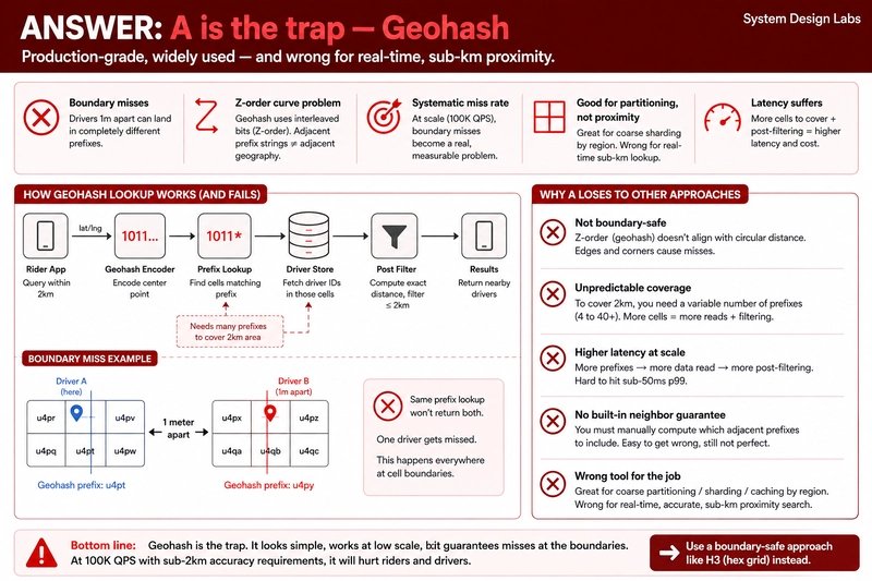
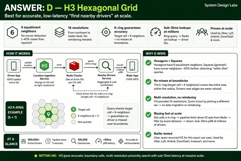
Uber's open-source H3 divides the earth into hexagonal cells across 16 resolution levels. Each hexagon has 6 neighbors, all equidistant from the center.

Why hexagons matter: Squares have corner neighbors that are approximately 40% farther than edge neighbors. This distorts radius-based proximity queries. Hexagons provide uniform neighbor distances, making "within 2km" queries geometrically accurate.

The killer feature: The k-ring query (target cell + 6 neighbors) guarantees no driver gets missed near cell boundaries. You fetch cell IDs from Redis sets keyed by cell, achieving sub-10ms lookups at millions of drivers.

Uber built this for exactly this problem. Lyft, Airbnb, and DoorDash all use variants.

The Production Reality

At scale, the answer is usually a combination. H3 provides the spatial indexing layer. Redis provides the low-latency storage for real-time updates. The write path handles driver location updates by computing H3 cell IDs and updating Redis sets. The read path computes the query cell's k-ring, fetches driver IDs from Redis, and returns results.

The key insight: spatial indexing at scale isn't about choosing the perfect data structure. It's about minimizing write amplification while maintaining query accuracy. H3's hexagonal geometry and fixed resolution levels solve the boundary problem that plagues grid-based approaches.

Trade-offs Worth Considering

Approach	Write Cost	Query Accuracy	Boundary Handling	Operational Complexity
Geohash	Low	Poor at boundaries	Systematic misses	Low
PostGIS	High (GiST writes)	Perfect	Correct	Medium
Quadtree	Medium (rebalancing)	Good	Boundary churn	High
H3	Low (cell assignment)	Very Good	K-ring solves it	Medium

The pragmatic choice depends on your scale and accuracy requirements. Below 50,000 active drivers, PostGIS might be sufficient. Above that, H3 + Redis becomes the standard architecture.

Implementation Patterns

If you're building this today, the architecture looks like:

1. Write path: Driver GPS update → compute H3 cell ID at resolution 9 (average edge length 174m) → update Redis set for that cell → publish to real-time stream
2. Read path: Rider query → compute H3 cell for rider location → compute k-ring (1 ring for 2km radius at resolution 9) → fetch driver IDs from Redis → return sorted by actual distance
3. Consistency: Accept eventual consistency for driver positions. A 5-second staleness window is acceptable for ride-hailing.

The real engineering challenge isn't the spatial index itself. It's handling the operational reality: driver GPS drift, network partitions causing stale positions, and graceful degradation when Redis clusters experience failover.

Bottom Line

Choose D (H3) for new implementations at scale. The hexagonal geometry solves real problems that rectangular grids create. The H3 documentation and Uber's engineering blog provide production-tested implementation guidance.

If you're already running PostGIS successfully below 50,000 drivers, don't rewrite. Add H3 as a read-optimized layer alongside your existing system. Migrate gradually as scale demands.

The worst mistake is choosing based on theoretical elegance rather than production constraints. Every spatial indexing decision at scale is a trade-off between write amplification, query accuracy, and operational complexity. Choose based on which trade-off your system can absorb.