When Small Delays Don't Change Everything: The Surprising Stability of Differential Equations

Differential equations form the backbone of mathematical modeling across science and engineering, describing everything from population dynamics to electrical circuits. Most students encounter these equations in their standard form, where the rate of change at any moment depends only on the current state. But there's a fascinating variant that introduces memory into the system: delay-differential equations (DDEs).

In a delay-differential equation, the rate of change depends not just on the present state but also on the system's state at some earlier time. This seemingly small modification can dramatically alter the behavior of solutions, introducing oscillations, instabilities, and entirely new dynamical phenomena. Yet remarkably, under certain conditions, these delays can be so small that they don't change the fundamental character of the solution at all.

Consider the simple first-order delay-differential equation:

x′(t) = a x(t) + b x(t − τ)

Here, x′(t) represents the rate of change at time t, x(t) is the current state, and x(t − τ) is the state τ units of time ago. The constants a and b are non-zero real numbers, while τ is a positive delay. At first glance, introducing this delay term might seem like it would fundamentally alter the system's behavior. After all, we're now accounting for the system's memory of its past state.

However, a theorem proven by Driver, Sasser, and Slater in 1973 reveals a surprising truth: if the delay τ is sufficiently small, the qualitative behavior of this equation remains unchanged from the case where τ = 0 (no delay at all). Specifically, the equation behaves the same way provided:

-1/e < bτ exp(−aτ) < e

and

aτ < 1

The first condition involves a product of the delay, the coefficient b, and an exponential term that depends on a. The second condition simply requires that the product of a and τ remains less than one. These constraints define a region in the (a, b, τ) parameter space where the delay is "small enough" to not qualitatively alter the system's behavior.

This result has profound implications for modeling real-world systems. Many natural and engineered systems exhibit delayed responses—chemical reactions with transport delays, population dynamics with maturation periods, control systems with sensor lag. The theorem suggests that if these delays are sufficiently small relative to the system's intrinsic time scales (captured by the coefficients a and b), we can often approximate the delayed system with a simpler, non-delayed model without losing essential insights about its behavior.

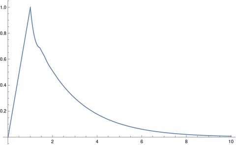
To illustrate, consider the specific example:

x′(t) = −3 x(t) + 2 x(t − τ)

with initial condition x(1) = 1. Without any delay (τ = 0), this equation has the simple solution x(t) = exp(1 − t), which monotonically decays to zero. The theorem predicts this same qualitative behavior should persist as long as the delay satisfies our conditions. For this particular equation, that means τ < 0.404218.

When we solve this equation numerically for τ = 0.4 using computational tools like Mathematica, we indeed observe the solution eventually decaying monotonically to zero, just as in the non-delayed case. The initial behavior might differ slightly due to the specified initial history function, but the long-term qualitative behavior matches.

However, when we increase the delay to τ = 3 and rerun the simulation, the solution exhibits oscillations—a qualitatively different behavior that violates the theorem's conditions. This dramatic change illustrates how delays beyond the "small enough" threshold can fundamentally alter system dynamics.

One subtle aspect of delay-differential equations is that they require more information to specify a unique solution than ordinary differential equations. While an ordinary differential equation needs only an initial condition like x(0) = x0, a delay-differential equation requires specifying the solution over an entire interval of length τ before the initial time. This "history function" can be any function of t (subject to certain technical conditions) defined on the interval [−τ, 0].

The mathematical machinery behind these results involves careful analysis of the characteristic equation associated with the delay-differential equation and sophisticated techniques from functional analysis. The proof demonstrates that for sufficiently small delays, the spectrum of the associated linear operator remains in the left half of the complex plane, ensuring stability.

This theorem and its generalizations have found applications in various fields. In control theory, it helps determine when delayed feedback can be safely ignored in system design. In population dynamics, it suggests when maturation delays can be neglected in modeling growth. In pharmacokinetics, it indicates when drug absorption delays are too small to affect the overall concentration profile significantly.

The beauty of this result lies in its counterintuitive nature: adding complexity (the delay term) doesn't necessarily make the system more complex in terms of its qualitative behavior. Under the right conditions, the system's memory of its past state doesn't fundamentally alter its future trajectory. This principle—that sufficiently small perturbations or modifications don't change qualitative behavior—appears throughout mathematics and physics, from perturbation theory in quantum mechanics to stability analysis in dynamical systems.

For practitioners, this theorem offers both theoretical insight and practical guidance. It provides a rigorous criterion for when delayed models can be safely approximated by simpler non-delayed ones, potentially saving significant computational effort while preserving essential insights. Conversely, it warns when delays are large enough to warrant the full complexity of delay-differential equation modeling.

The next time you encounter a system with small delays—whether in engineering design, biological modeling, or economic forecasting—remember that these delays might not be as consequential as they first appear. Sometimes, the simplest model is not just the easiest to work with, but also the most accurate representation of reality.